Example reduction
To confirm that the PIPPIN installation was successful and as an introduction to the pipeline, we provide an example reduction of the Ks-band observations of HD 135344B, observed as part of ESO programme 089.C-0611(A). This dataset was previously published in Garufi et al. (2013).
To run the example reduction, navigate to any directory in the terminal and type:
pippin_naco --run_example
PIPPIN attempts to locate the required data in the current directory. If these files do not exist, they can be automatically downloaded from the GitHub repository (48.4 MB). After successfully downloading the data, which includes SCIENCE, FLAT, and DARK observations, as well as a configuration-file with input parameters (config.conf), PIPPIN begins the reduction.
Note
A discussion of the input parameters in config.conf can be found here.
As the pipeline is running, information is printed in the terminal and stored in the example_HD_135344B/pipeline_output/log.txt file. First, the FLATs and DARKs are median-combined into master FLATs and master DARKs per observation type. The master FLATs are normalized to unity. Master bad-pixel masks (BPMs) are created from the non-linear pixel response between FLAT observations with the FLAT-lamp on or off.
The parameters in the configuration-file are read and the SCIENCE observations are grouped by observation type (only one in this example). After DARK-subtraction and FLAT-normalisation, figures are generated in the example_HD_135344B/pipeline_output/200236070_0.3454_Ks/plots/ directory. These figures are updated once the sky-subtraction is performed and the ordinary and extra-ordinary beams are cropped out. The sky-subtraction is carried out by subtracting two observations with different nodding-positions from each other.
The PDI method is applied to the cropped-out beams and a series of corrections are performed to mitigate the effects of instrumental polarisation. The final data products are stored in the example_HD_135344B/pipeline_output/200236070_0.3454_Ks/PDI/ directory. Running the following command within a terminal in the example_HD_135344B/pipeline_output/200236070_0.3454_Ks/PDI/ directory will show the \(Q_\phi\) and \(U_\phi\) images in DS9.
ds9 -tile -mecube Q_phi.fits -cube 7 -scale limits -10 40 U_phi.fits -cube 7 -scale limits -5 20 -lock frame wcs -lock colorbar yes -cmap cool
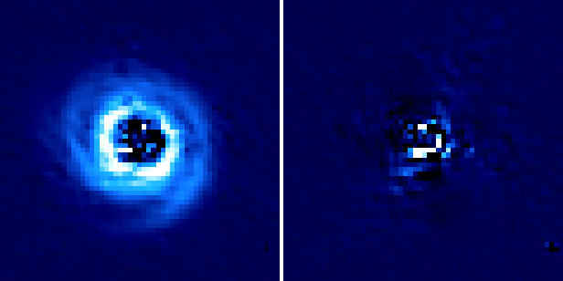
The left figure shows the \(Q_\phi\) image and the right figure displays the \(U_\phi\) signal. The images above show the result of only 2 HWP cycles and thus have a lower signal-to-noise than the combination of all 16 cycles. Since the crosstalk_correction and minimise_U_phi parameters were set to True in the configuration file, the 7th extension of the Q_phi.fits and U_phi.fits (displayed in DS9 with the command above) show the data products with the highest level of instrumental polarisation correction (i.e. IP-subtraction, crosstalk-correction and \(U_\phi\)-minimisation).
In the next section we will learn how to reduce other NACO polarimetric datasets.